
Segmentation
Semantic Segmentation
- 모든 pixel에 label을 할당하는 것 (one label per pixel)
- instance를 구분하지 않음
- class의 수는 보통 정해져 있음
Instance Segmentation
- instance를 detect하고, 각각의 pixel에 label을 부여하여 instance를 구분함.
- "simultaneous detection and segmentation" (SDS)라고 불리기도 함.
Semantic Segmenation
이미지 input -> 특정 patch를 추출 -> cnn에 돌림 -> 가운데 픽셀이 분류됨
=> 이 과정들을 모든 pixel에 반복함
하지만, 이 방법은 비용이 너무 많이 드는 문제가 있음.
patch를 사용하는 것 대신 fully convolutional network를 사용하여 모든 픽셀을 한번에 얻는 방법을 사용함.
그런데 이 방법은 pooling layer 로 크기가 작아지는 문제가 있음.
Segmantic Segmentation : Multi-Scale
여러개의 스케일을 사용하는 아이디어.
이미지를 다양한 스케일로 resizing (마치 이미지 피라미드와 같음) -> 스케일링된 이미지를 각각의 CNN으로 돌려줌 -> 모두 원본과 같은 크기로 upsampling하고 concatenate 과정을 거침
이미지를 외부에서 "bottom-up" segmentation 과정을 거침(super pixels or segmentation tree)
=> 두 과정을 결합시켜 최종 output을 완성시킴
Segmantic Segmentation : Refinement
이미지를 RGB 3개의 채널로 분리된 상태로 cnn에 적용해 모든 label을 얻어낸다 -> 그 결과에 다시 한번 cnn 적용 -> 다시 적용
(이 3번의 과정에서 cnn은 parameter를 sharing 하고 있다.)
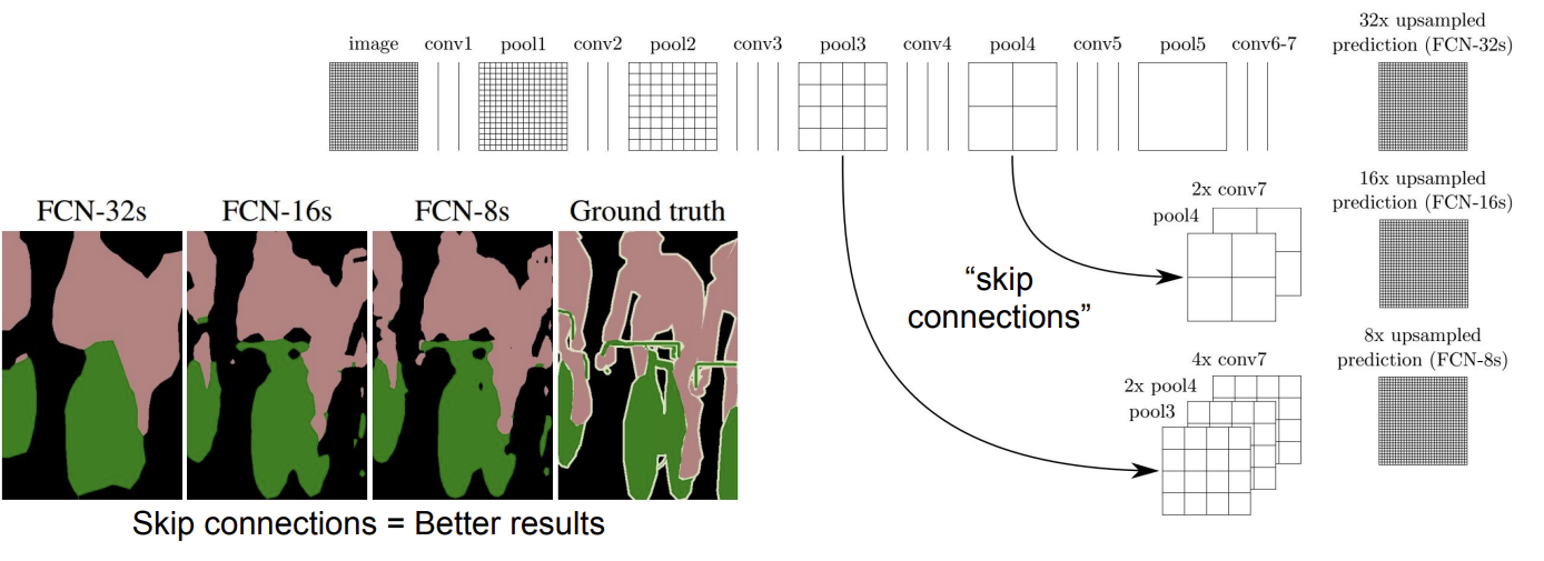
Segmantic Segmentation : Upsampling
작아진 feature map을 복원해주는 upsampling 방법에서 기존에는 별도의 작업을 사용했지만, 이 방법에서는 upsampling 과정까지도 network에 포함시킴. 즉, 학습이 가능한 upsampling layer가 등장한 것.
또한 skip connection 과정을 통해 앞단의 pooling layer를 가져와 통합시켜 성능을 향상시킴.
Learnable Upsampling : "Deconvolution"
위와 같이 학습할 수 있는 upsampling 방법을 Deconvolution 이라고 부르기도 한다.
일반적인 convolution의 결과는 dot product를 통해 다음과 같은 output이 도출될 것이다.
(4-3+2x1)/1 +1 = 4

Deconvolution은 weight을 부여하는 과정을 통해 upsampling을 한다.
겹치는 부분은 sum 연산으로 처리한다. convolution에서의 backward pass와 동일하다.
즉, deconv의 forward pass = conv의 backward pass
deconv의 backward pass = conv의 forward pass 와 동일한 과정이다.
그래서, 사실 "inverse of convolution"이 정확한 표현이다.

Instance Segmenation
오래전부터 연구되어오던 Semantic segmentation과 달리 instance segmentation은 비교적 최근 연구 주제이다.
R-CNN과 비슷한 방식이다.
external segment proposal을 진행하고, 이를 통해 feature를 뽑아내어 box CNN에 돌려 bounding box를 얻어낸다.
동시에 mean image를 사용해 background를 제거한 이미지를 Region CNN에 돌린다.
두 결과물을 Region에 대해 분류를 진행한다. 마지막으로 Region refinement 과정을 거친다.

Instance Segmentation: Hypercolumns
원본이미지를 crop하여 alexnet에 돌리고, conv과정에서 upsampling 을 적용해 combine하여 결과를 도출한다.

Instance Segmentation: Cascades
Faster R-CNN과 매우 유사하다.
이미지 자체를 convolution 시켜 거대한 feature map을 만들어내고 RPN을 이용해 ROI를 뽑아낸다.
생성된 box를 warping과 pooling으로 동일한 사이즈로 맞춰주고 FC에 돌린다. 그 후 figure / ground logistic regression을 이용해 mask instances를 생성한다. 그 후 masking 과정을 통해 background를 제거하고 FC에 돌려 object의 class을 분류해낸다.
모든 과정은 end-to-end로 학습 시킬 수 있다.

Semantic segmentation
○ Classify all pixels
○ Fully convolutional models, downsample then upsample
○ Learnable upsampling: fractionally strided convolution
○ Skip connections can help
● Instance Segmentation
○ Detect instance, generate mask -> detection의 R-CNN, Faster R-CNN과 유사한 개념들이 등장
○ Similar pipelines to object detection
Attention Models
Recall : RNN for captioning
해당 방법은 RNN이 전체의 이미지를 한번만 보게되는 한계점이 존재, 따라서 RNN이 매 timestep 마다 이미지의 다른 부분을 보는 방법이 등장하게 됨.

그 방법이 바로 Soft Attention for Captioning
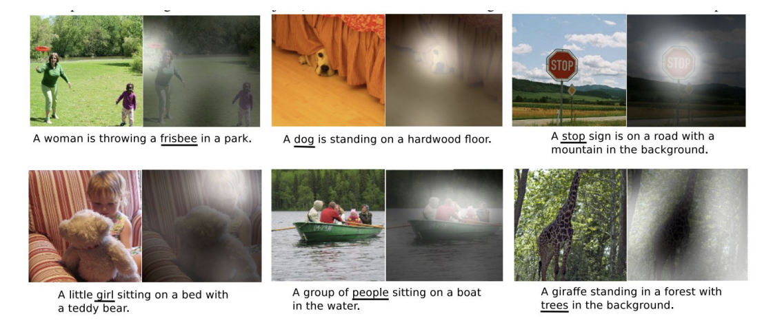
Soft Attention for Captioning
FC layer에서 나온 single feature가 아닌 그 전의 feature grid를 사용
이를 h0을 초기화 하는데 사용, a1(location에 대한 확률 분포)을 바로 추출, 이 확률 분포를 feature와 연산하여 weighted feature를 계산함. 이는 single summarization vector가 됨. 이를 생성하는 방법에는 2가지 방법이 존재
바로, soft attention, hard attention이다.

Soft vs Hard Attention
soft attention에서는 모든 location을 고려함. gradient descent를 사용하는데 적합 -> end-to-end 학습 가능
=> 연산량이 많음
hard attention에서는 가장 높은 확률을 가지는 grid를 선택, gradient descent를 사용할 수 없음. -> 별도의 강화학습 필요
=> 연산량이 적고, 정확도가 높음

결과
정해져 있는 grid에 대한 attention만 가능하다는 문제점 존재
-> 임의의 지점에 attention을 주는 방법 등장

Attending to Arbitrary Regions : DRAW

Attending to Arbitrary Regions : Spatial Transformer Network
localize 후 좌표를 생성, 그 후 crop하여 rescale 과정을 거침.
이를 함수라고 한다면 이를 미분가능한 함수를 만들 수 있을까?
input의 픽셀 좌표를 output의 픽셀 좌표로 mapping 해주는 함수를 생성
이를 통해 sampling grid를 생성, 그 후 bilinear interpolation으로 최종 결과물을 얻을 수 있음


Soft attention:
○ Easy to implement: produce distribution over input locations, reweight features and feed as input
○ Attend to arbitrary input locations using spatial transformer networks
Hard attention:
○ Attend to a single input location
○ Can’t use gradient descent!
○ Need reinforcement learning!
'컴퓨터비전' 카테고리의 다른 글
| [CS231n 2016] 11강 CNNs in Practice (0) | 2022.07.21 |
|---|---|
| [CS231n 2016] 10강 Recurrent Neural Networks (0) | 2022.07.18 |
| [CS231n 2016] 9강 Understanding and Visualizing Convolutional Neural Networks (0) | 2022.07.15 |
| [CS231n 2016] 8강 Spatial Localization and Detection (0) | 2022.07.14 |
| [CS231n 2016] 7강 Convolutional Neural Network (0) | 2022.07.11 |


