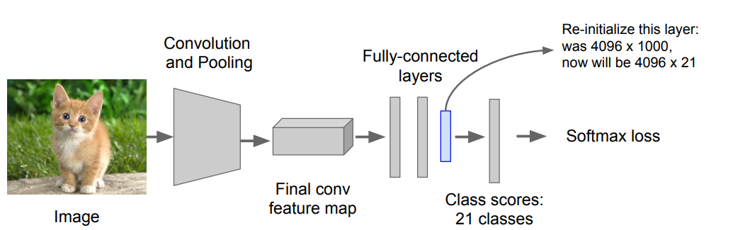
- Throw away final fully-connected layer, reinitialize from scratch
- Keep training model using positive / negative regions from detection images
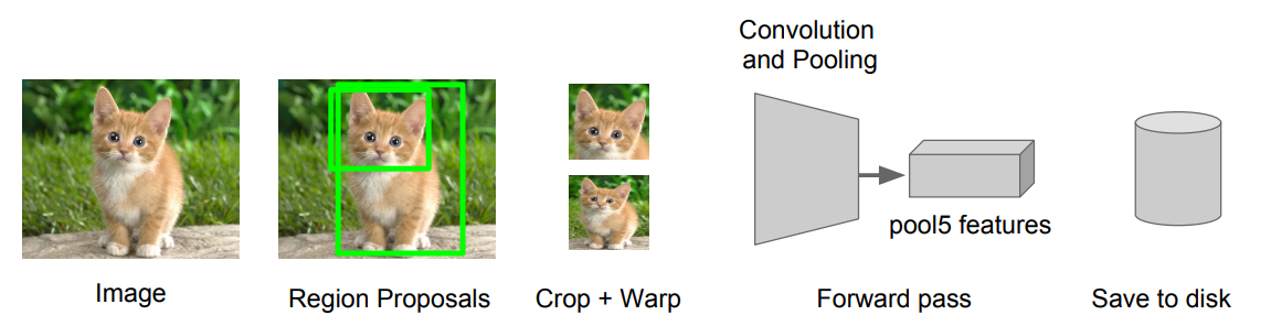
Step 3: Extract features
- Extract region proposals for all images
- For each region: warp to CNN input size, run forward through CNN, save pool5 features to disk
- Have a big hard drive: features are ~200GB for PASCAL dataset!
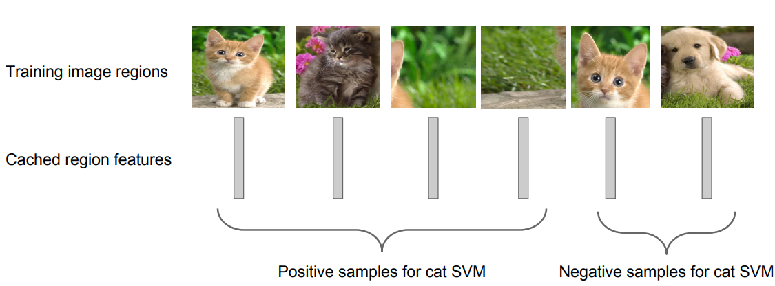
Step 4: Train one binary SVM per class to classify region features
ex) 고양이라면, 고양이인지? 아닌지? 2개 중 하나로 positive, netgative 분류를 함.
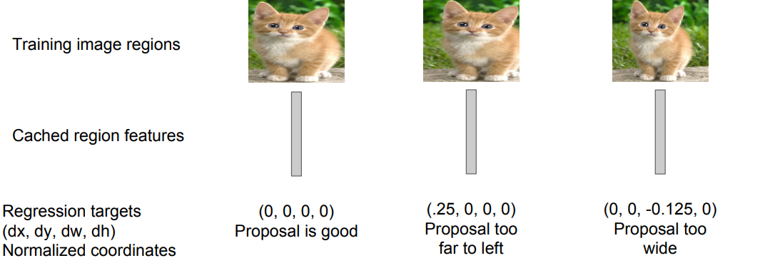
Step 5 (bbox regression): For each class, train a linear regression model to map from cached features to offsets to GT boxes to make up for “slightly wrong” proposals
(region proposal이 항상 정확한 것은 아니기 때문에, cache 해놓은 feature에서 regression을 이용해 정확도를 높혀주는 작업이다. 이는 mAP를 3~4% 정도 높혀준다.
Object Detection : Datasets
PASCAL VOC, ImageNet Detection, MS-COCO...
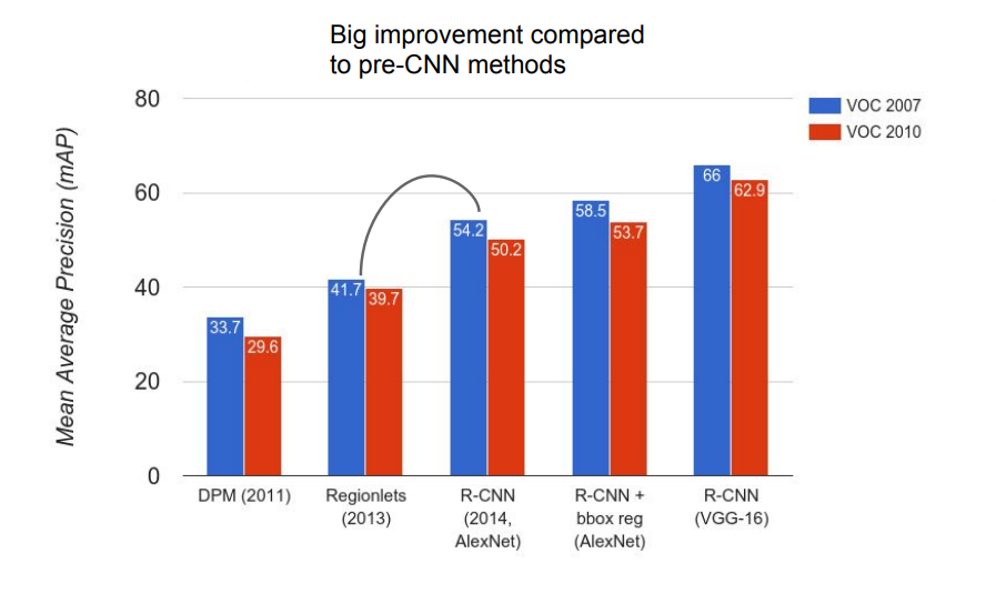
Object Detection : Evaluation
mean average precision (mAP)
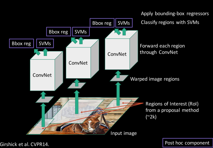
R-CNN의 문제점
1. Slow at test-time: need to run full forward pass of CNN for each region proposal
2. SVMs and regressors are post-hoc: CNN features not updated in response to SVMs and regressors
3. Complex multistage training pipeline
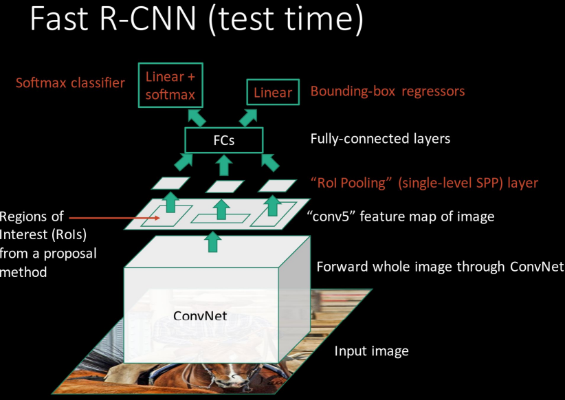
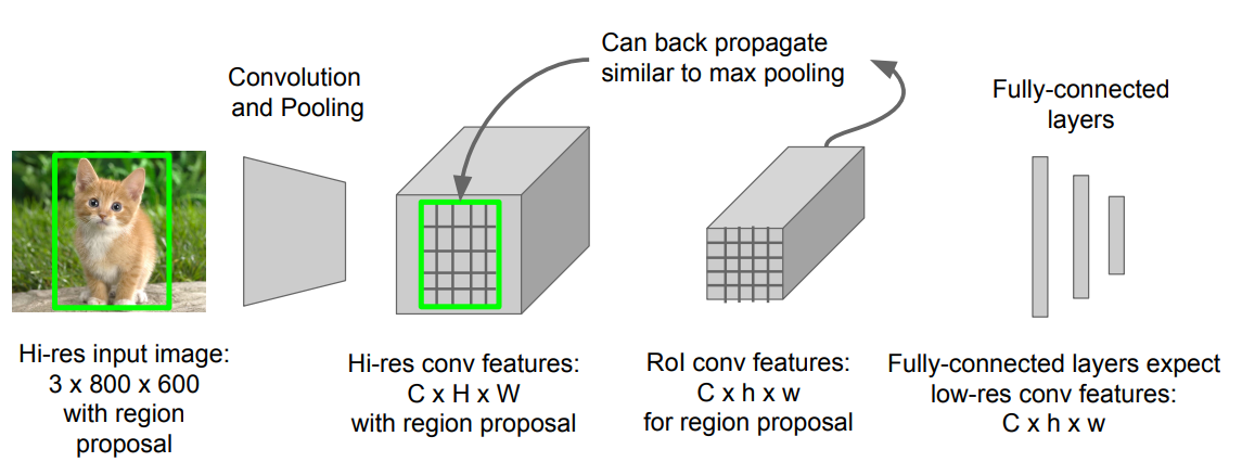
Fast R-CNN
CNN과 region proposal 추출의 순서를 바꾼 것
이미지를 우선 CNN에 돌려 고해상도의 conv feature map을 생성한다.
여기서 proposal method를 사용해 ROI를 추출하고, 이를 ROI Pooling이라는 기법을 사용해
FC layer로 넘겨줘 classifier와 regression을 수행한다.
R-CNN Problem #1: Slow at test-time due to independent forward passes of the CNN
Solution: Share computation of convolutional layers between proposals for an image
R-CNN Problem #2: Post-hoc training: CNN not updated in response to final classifiers and regressors
R-CNN Problem #3: Complex training pipeline
Solution: Just train the whole system end-to-end all at once!
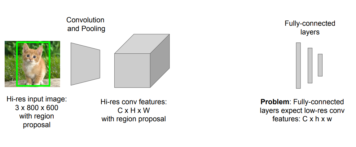
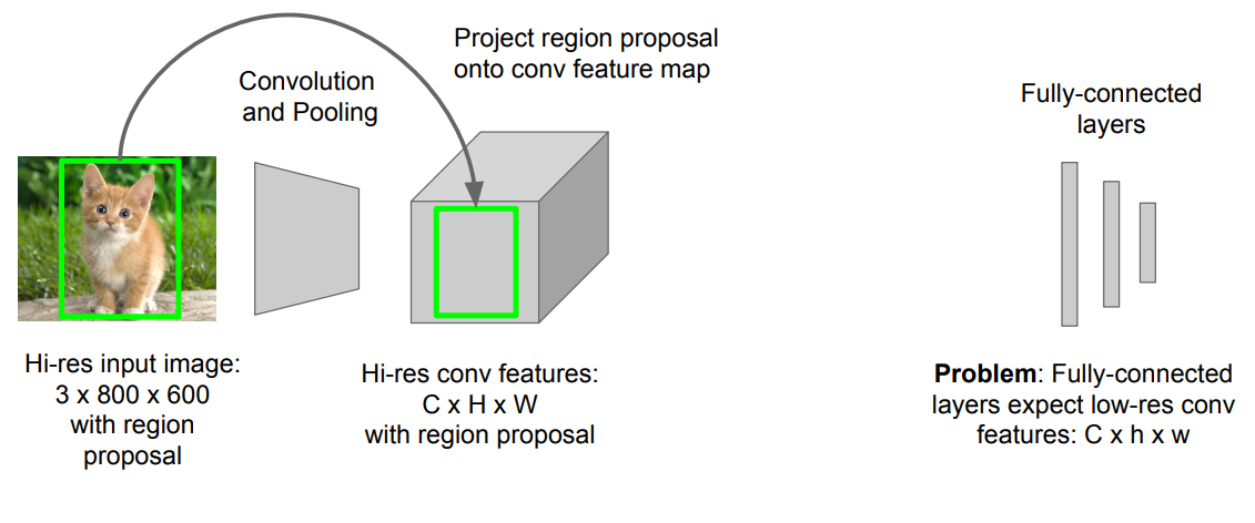
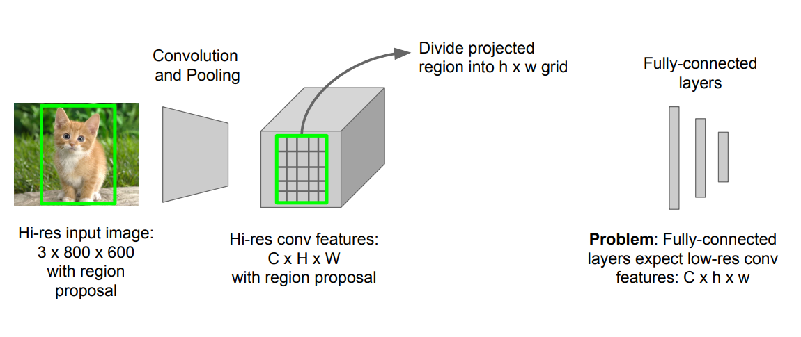
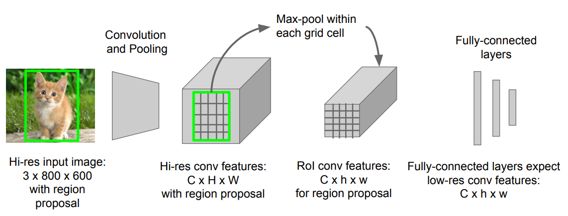
high-res conv feature = > low-res conv feature로 바꿔주는 것을 ROI Pooling이 해결해주게 됨.
ROI Pooling의 과정
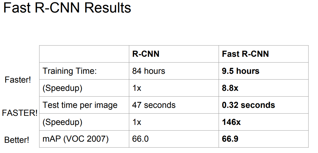
Fast R-CNN 결과
R-CNN은 각각의 Region proposal에 대해 별개로 forward pass
Fast R-CNN은 Region proposal간의 conv layer의 computation을 share하기 때문에 빠르게 된다.
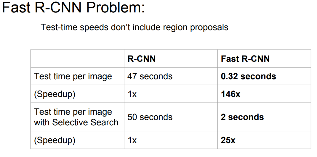
Fast R-CNN의 Problem
region proposal을 포함하게 되면 2초나 걸려 real-time으로는 사용하기 힘듬.
Fast R-CNN의 Solution:
Just make the CNN do region proposals too!
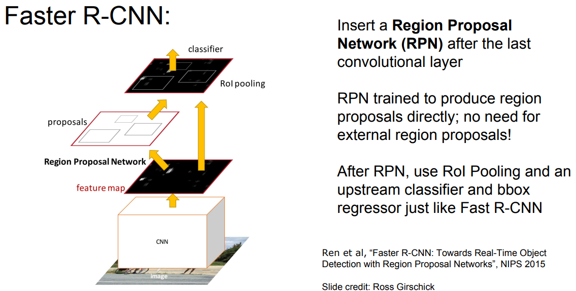
Faster R-CNN
이전까지는 Region Proposal을 외부에서 진행해왔음.
Region Proposal Network를 삽입하여 내부에서 Region Proposal을 수행하게 함.
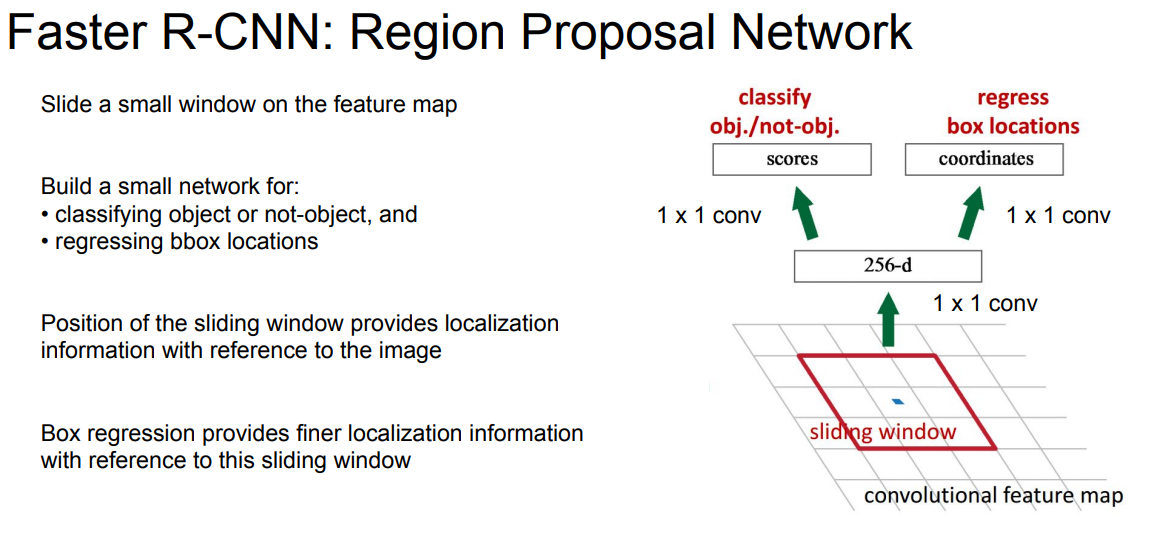
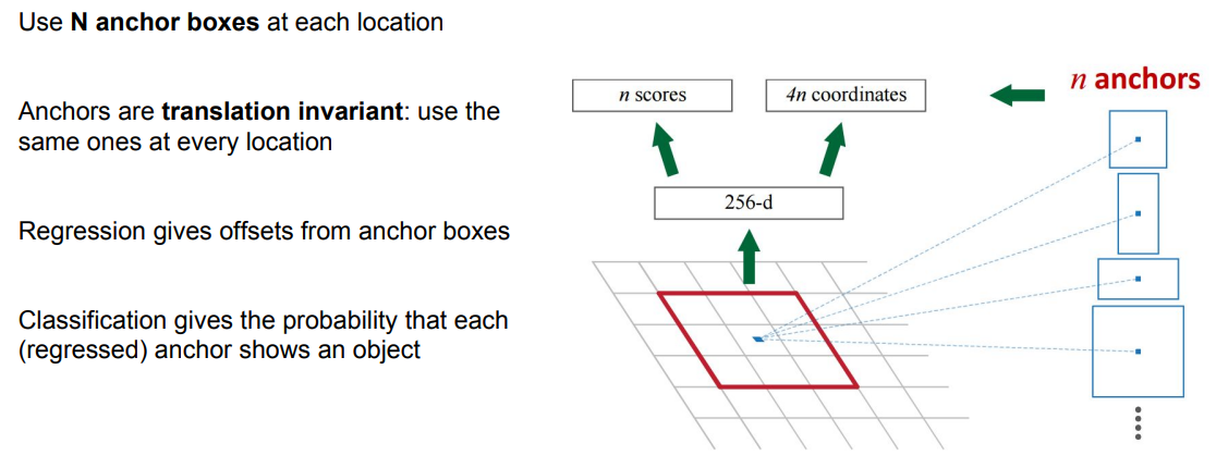
Faster R-CNN : Region Proposal Network
기본적으로 Convolution Net이다. sliding 3x3 window로 Region Proposal을 생성해냄.
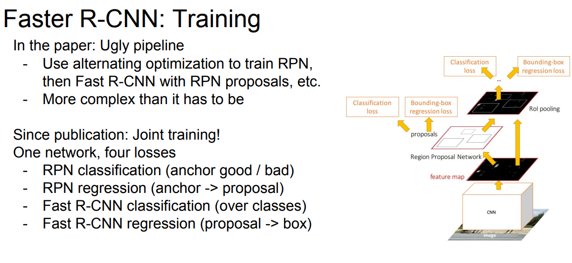
Faster R-CNN : Training
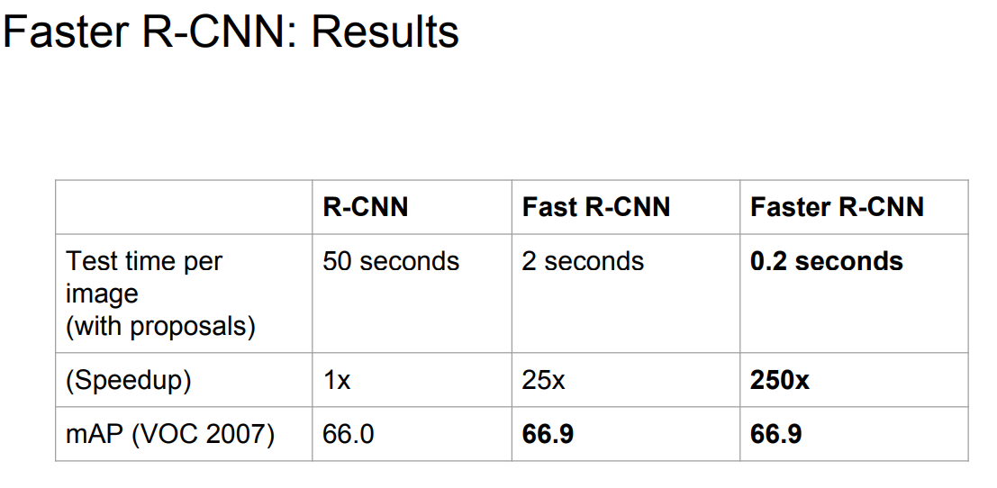
Faster R-CNN : Results
YOLO: You Only Look Once Detection as Regression
Detection을 Regression으로 간주하고 적용하는 기법 이전에는 Detection을 classification으로 간주했었음.
Divide image into S x S grid Within each grid cell(일반적으로 7x7)
predict: B Boxes: 4 coordinates + confidence Class scores: C numbers
Regression from image to 7 x 7 x (5 * B + C) tensor
Direct prediction using a CNN
Faster R-CNN 보다 빠르지만, 성능이 좋지는 않다.
Recap Localization:
- Find a fixed number of objects (one or many)
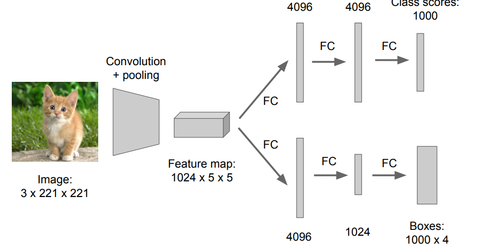
- L2 regression from CNN features to box coordinates
- Much simpler than detection; consider it for your projects!
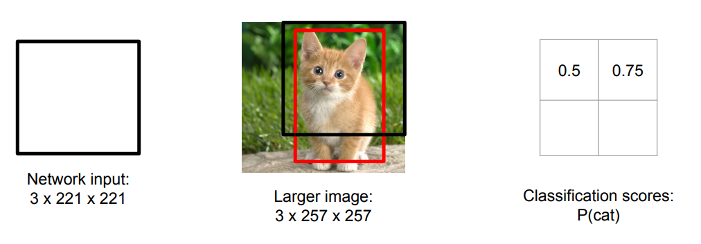
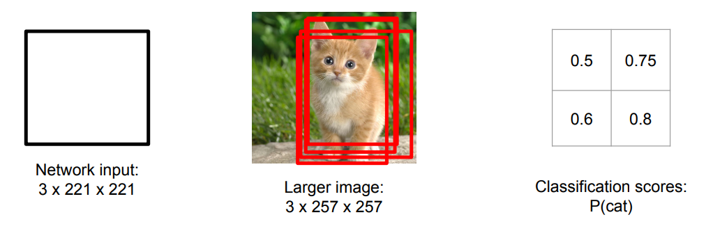
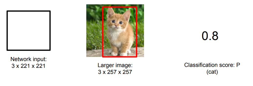
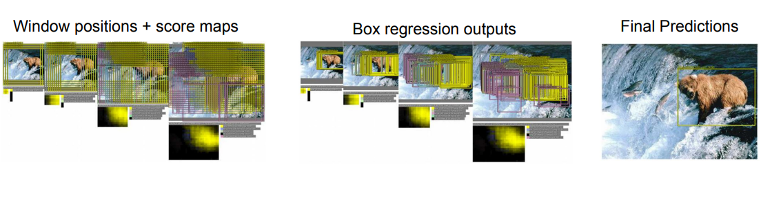
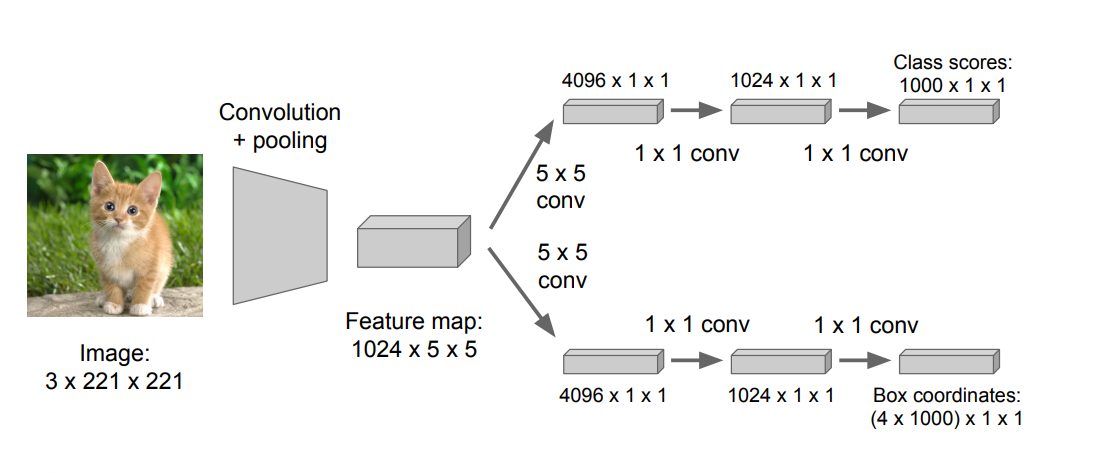
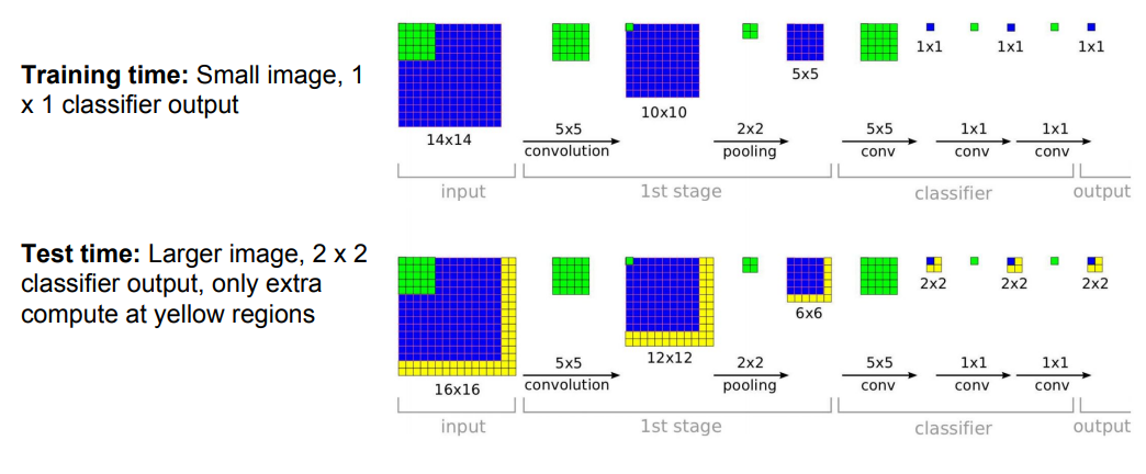
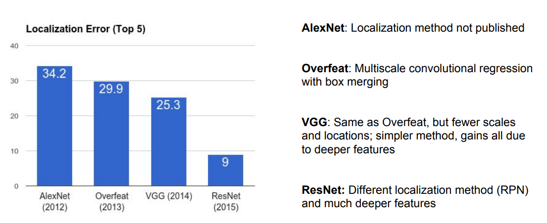
- Overfeat: Regression + efficient sliding window with FC -> conv conversion
- Deeper networks do better
Object Detection:
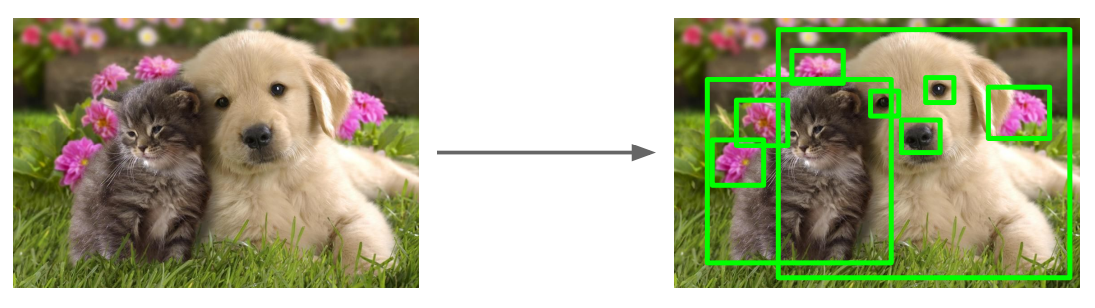
- Find a variable number of objects by classifying image regions
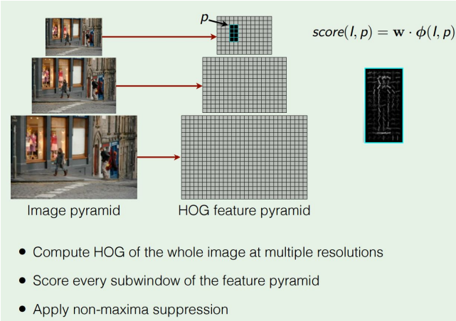
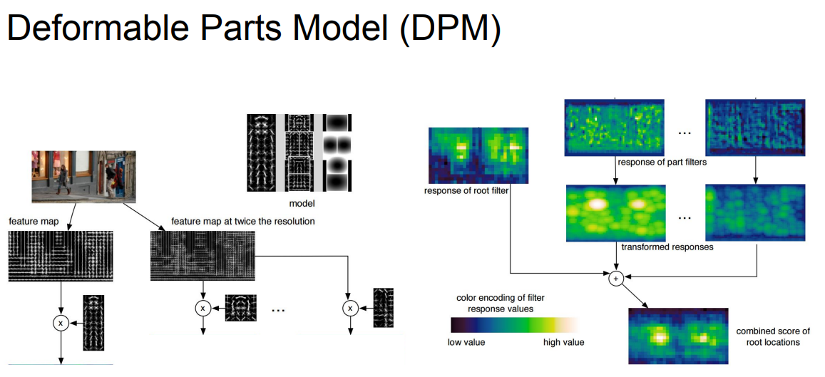
- Before CNNs: dense multiscale sliding window (HoG, DPM)
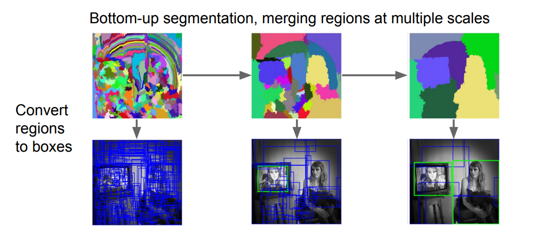
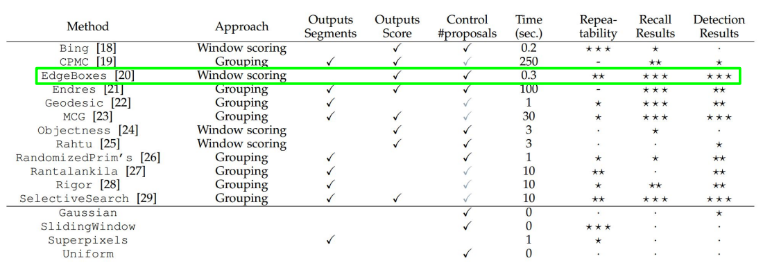
- Avoid dense sliding window with region proposals